Non-invasive loop design

Proportional-integral-derivative (PID) controllers are ubiquitous. Designing and tuning them may appear simple in theory, but it can be difficult and time consuming in practice. A common method of tuning PID controllers is to manually adjust controller gains while the controller runs the plant. This time-consuming method requires access to the plant hardware and can lead to plant damage if chosen gain values result in unstable plant behaviour. Using model-based design, the development process can be improved by systematically designing, testing and implementing PID controllers on programmable logic controllers (PLCs), programmable automation controllers (PACs) and microprocessors.

With model-based design we use a block-diagram environment to create system models of the plant and controller. These models can be simulated, allowing us to quickly iterate and refine controller design before it is implemented and deployed. The need for access to plant hardware is reduced because we can do a lot of testing through simulations instead of involving the plant. Early verification through simulation ensures that the controller performs as expected when deployed to the actual plant.

Model-based design of PID controllers involves the following four steps: Creating the plant model Designing the PID controller Testing the controller in real time Implementing the design Using a digital motion control system as an example, we describe how to apply model-based design for rapid design and prototyping of a PID controller. Digital motion control system Our example plant consists of a power amplifier driving a DC motor and two rotary optical encoders for measuring the position of the motor shaft and the load. The motor is connected to the load through a small flexible shaft to approximate the compliance found between the actuator and the load in many motion control systems. The control system ensures that the load follows the specified trajectory by measuring the error between the required and measured load angle. It then uses a PID controller to calculate and send a voltage request to the motor. Our design is to improve machine performance from the current maximum speed of 150 rad/s and acceleration of 2000 rad/s2 to new speed and acceleration targets of 250 rad/s and 5000 rad/s2, respectively. We want to achieve these performance gains without losing any position accuracy. Specifically, we want the error between commanded and measured load angle to be less than one degree. The existing controller design does not meet the new performance specifications, as shown in Figure 1. Our aim is to acheive the response shown in Figure 2. Instead of manually tuning PID gains on the actual plant hardware, we can use model-based design to develop, test and implement the controller. Creating the plant model There are two primary approaches for creating a plant model: data-driven modelling and first-principles modelling. With data-driven modelling we create a plant model that fits measured input-output test data. We want to operate the controller during data collection to ensure minimal disruption of plant operation. To collect the input-output data, we add as our input signal a random white-noise signal onto the voltage fed to the DC motor.		Figure 1: Old controller design with a maximum position error of more than 4° (bottom) when trying to follow a reference trajectory (top) corresponding to new speed and acceleration targets.
		Figure 2: System response for desired reference trajectory. The new controller design has an error of less than 1.

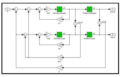
Our output signal is the overall voltage that the controller sends to the DC motor. After we collect this input-output data, we can calculate the frequency response of the closed-loop system. And because we know the exact gains in our current controller design (the one we are trying to improve), we can obtain the frequency response of the plant. Finally, to be able to simulate our controller in the time domain, we use the frequency response of the plant to estimate the plant transfer function using system identification techniques, as shown in Figure 3. With first-principles modelling we create the underlying dynamic equations of the plant using standard block-diagram modelling by connecting together gain, summation and integrator blocks (Figure 4).

Figure 3: Estimated plant frequency response and plant transfer function model obtained using system identification.

When modelling mechanical and electrical systems it is often more convenient to create a plant model by taking physical properties of the system, such as inertia, stiffness, damping, resistance and inductance, and connecting them together, just as we would draw a mechanical diagram or electric circuit of the system. This variation of first-principles modelling technique, called physical modelling, enables us to create plant models without deriving the underlying equations of plant dynamics.

Figure 4: Block diagram model implementing dynamic equations of the plant.

Often it is beneficial to blend these two distinct modelling approaches (data-driven and first-principles). To do this, we use measured input-output data from the actual system to adjust parameters of the physical model. Parameters (motor and load inertias, stiffness and damping) are adjusted by using numerical optimisation techniques. We play the measured input through the model and compare the model output to the measured output from the actual system. We iteratively adjust model parameters until we get the best possible fit between the output of the calibrated model and measured output. This iterative adjustment can be completely automated using optimisation techniques.

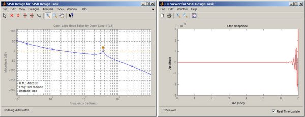
Designing the PID controller PID design and tuning is easy once the plant model is available. We add a PID controller block to the block diagram model of our plant to create a closed-loop system model. The PID controller block is parameterised with proportional, integral and derivative gains that need to be updated to achieve the desired system performance. Rather than manually tuning these gains, we use an automatic PID tuning method, shown in Figure 5, which automatically calculates PID gains for our plant model. To speed up our controller, we use an interactive slider for a faster response time. When we attempt to increase the controller speed, we notice that the system becomes unstable. Further analysis of the system in the frequency domain reveals a resonant peak that is causing unstable behaviour (Figure 6). Such instability is a well-known issue in motion control systems and is easily fixed by using a notch filter to cancel the resonance.

Figure 5: Automatic PID tuning. The PID tuner automatically calculates PID controller gains and allows interactive fine tuning with the slider to specify the desired response time.

We can add the notch filter by using the interactive control design tool that lets us interactively place a notch filter on top of the resonant peak. Doing this allows us to stabilise the system and increase controller speed. We now test our design (retuned PID controller and a notch filter) by running the nonlinear simulation of our closed loop system on our desktop. Running the simulation with the reference speed corresponding to the new desired system performance confirms that the new design meets the specifications, as shown in Figure 2.

Figure 6: Frequency response (left) and step response (right) of a closed-loop system with PIS controllers, showing resonant peak.

Use of simulation enables us to see the issue with the control system - increasing the PID gains in this case was not sufficient to meet the performance specifications. We need a notch filter to cancel the resonant peak. Automated PID tuning allows us to quickly find stabilising controller gains and finetune the design to meet desired performance targets. If we tried to tune our PID controller on the actual machine, we’d run into an unstable regime of operation that could have damaged our machine.

Testing the controller in real time

After the controller design has been validated via desktop simulation, the next step is to test the controller in real time. First we need to establish a real-time testing platform, which includes a real-time target computer with I/O boards. These I/O boards are typically connected to the actual sensors and actuators on the machine (or machine prototype). We now re-use our controller model and automatically generate C code for the PID controller and the notch filter, and then download this C code to the real-time target computer. We now have our controller code running in real time on the target computer and directly controlling the operation of the plant via inputs and outputs from plant sensors and actuators. Real-time testing lets us confirm that the entire system works properly under realistic conditions with realistic inputs and outputs before we go through the effort of implementing the controller on production hardware, such as PLCs or PACs. This is sometimes known as rapid control prototyping. We are also able to verify that real-time controller performance is still in line with what we observed in desktop simulation. If we find any discrepancies, we’re at an early enough stage in the development process to quickly and easily diagnose and fix the problem in the simulation model and then verify that the controller works properly in real time.

Implementing the design

Our last step is to deploy our controller to a target PLC, PAC or a microprocessor. We do that by automatically generating IEC 61131 structured text from our controller model. This structured text is generated in PLCopen XML and other file formats that are supported by widely used integrated development environments (IDEs). As a result, we can compile and deploy our controller to numerous PLC and PAC devices. If the final target is a microcontroller, we can instead automatically generate C code.

Conclusion

Plant modelling, closed loop simulation and automatic PID tuning allow us to tune and test our PID controller in desktop simulation. Our simulation model gives us the ability to identify a resonance in the system and to develop and test a notch filter to solve this problem. Real-time testing confirms that our control design matches desktop simulation results and meets design specifications. Implementation through automatic code generation means we are able to quickly implement our design on a PLC or microprocessor. Finally, the use of model-based design allows us to quickly develop, test and prototype our design, without damaging plant hardware or disrupting its operation.